IGRA+ decay sample size calculation

All the data and source code files are here.

You can ask report errors or for additional analysis here.

1 Packages

Needed packages:

needed_packages <- c(
  "dplyr",
  "bbmle",
  "purrr",
  "magrittr",
  "tidyr",
  "parallel",
  "whoami"
)

Installing the missing packages:

to_install <- needed_packages[! needed_packages %in% installed.packages()[,"Package"]]
if (length(to_install)) install.packages(to_install)

Loading packages:

library(dplyr)
library(bbmle)
library(purrr)
library(magrittr)
library(parallel)

2 Utility functions

Tuning abline():

abline2 <- function(...) abline(..., col = "lightgrey")

The logit function:

logit <- function(x) log(x / (1 - x))

The logistic function:

logistic <- function(x) 1 / (1 + exp(- x))

Random draws following the Bernoulli law:

rbern <- function(p) rbinom(length(p), 1, p)

A tuning of the runif() function:

runif2 <- function(max_t_before) runif(length(max_t_before), 0, max_t_before)

Below is a function that adds to a dataframe colones of proportion estimates together with borders of a confidence interval from a column x of successes and a column n of trials. This is a wrapper around the prop.test() function.

add_prop_est <- function(df, x, n, p = "est", l = "lwr", u = "upr", ...) {
  df |> 
    mutate(test   = map2({{ x }}, {{ n }}, prop.test, ...),
           "{p}" := map_dbl(test, ~ .x[["estimate"]]),
           conf   = map(test, ~ setNames(.x[["conf.int"]], c(l, u)))) |> 
    tidyr::unnest_wider(conf) |> 
    select(- test)
}

3 A simulator

A function that simulates data according to an exponential decay:

simulator <- function(p0, p1, t, t_entry, t_exposure = 0) {
  tibble(time = t_entry,
         igra = rbern(p0 * exp(log(p1 / p0) * (t_entry + t_exposure) / t)))
}

Where p0 is the assumed initial proportion of IGRA+, p1 is the assumed proportion of IGRA+ t years later initial time, t_entry is a vector of sampling times (i.e. dates of entry in the country) and t_exposure is a vector of the time before entry at which exposure happened. Note that:

both t_entry and t_exposure are vectors of random values
the number of samples corresponds to the length of t_entry
the length of t_exposure is either equal to 1 or the number of samples

An example with 500 samples showing what the simulations look like:

simulator(.3, .1, 10, runif(500, max = 10))

# A tibble: 500 × 2
    time  igra
   <dbl> <int>
 1 2.20      0
 2 4.39      1
 3 6.78      1
 4 0.146     0
 5 2.24      0
 6 8.66      0
 7 6.11      0
 8 1.34      1
 9 8.30      0
10 9.78      0
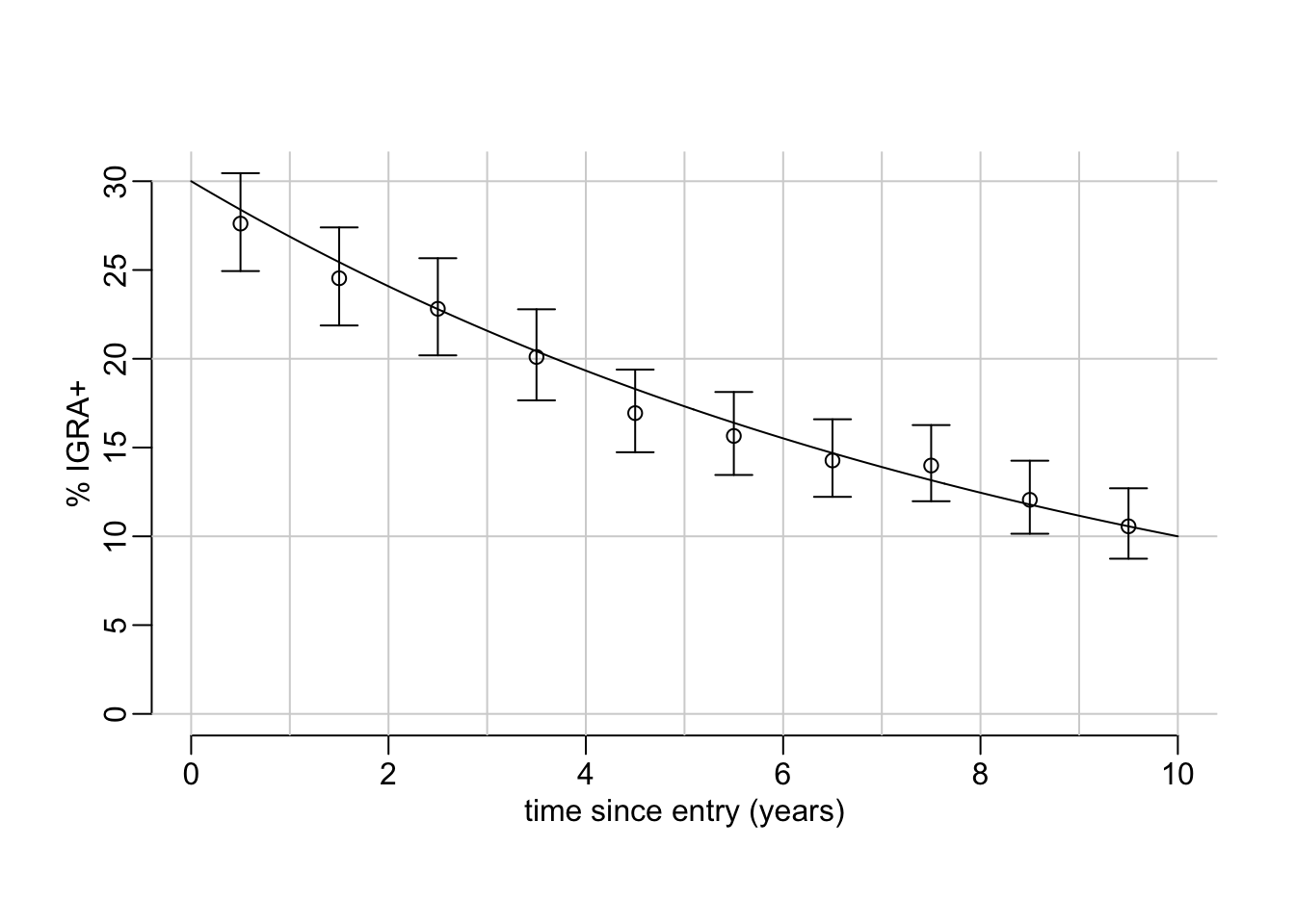
# ℹ 490 more rows

To explore a bit the simulations, let’s create a function that ease the vizualization of the Bernoulli trials data:

show_simulations <- function(simulations, xlim = c(0, 10), breaks = 0:10) {
  simdata <- simulations |> 
    mutate(time2 = cut(time, breaks)) |> 
    group_by(time2) |> 
    summarise(x = sum(igra), n = length(igra)) |> 
    add_prop_est(x, n) |> 
    mutate_at(c("est", "lwr", "upr"), multiply_by, 100) |> 
    mutate(time = as.integer(time2) - .5)

  plot(NA, xlim = xlim, ylim = c(0, max(simdata$upr)),
       xlab = "time since entry (years)", ylab = "% IGRA+")
  abline2(h = 10 * 0:10); abline2(v = 0:max(xlim))
  
  with(simdata, {
    points(time, est)
    arrows(time, lwr, time, upr, .1, 90, 3)
  })
}

And let’s build the following wrapper around this function:

explore_simulations <- function(p0 = .3, p1 = .1, t = 10, n = 1000,
                                xlim = c(0, 10), breaks = 0:10) {
  show_simulations(simulator(p0, p1, t, runif(n, max = t)), xlim, breaks)
  xs <- seq(0, t, le = 500)
  lines(xs, 100 * p0 * exp(xs * log(p1 / p0) / t))
}

Let’s play with it:

explore_simulations(p0 = .3, p1 = .1, t = 10, n = 10000)

4 Exponential decay model

4.1 ML estimation

Let’s write down the minus log-likelihood of the exponential decay model:

mLL <- function(logita, logmlambda, time, igra) {
  p <- logistic(logita) * exp(- exp(logmlambda) * time)
  igra <- as.logical(igra)
  - sum(log(c(p[igra], (1 - p)[! igra])))
}

Where logitsa is the logit value of the initial proportion of IGRA+, logmlambda is the log of minus the rate of decay and time and igra are the columns of the simulation dataframe. Let’s generate some simulations:

simulations <- simulator(.3, .1, 10, runif(500, max = 10))

And let’s use these simulated data to compute the likelihood of the exponential decay model:

mLL(logit(.3), log(- log(.1 / .3) / 10), simulations$time, simulations$igra)

[1] 225.9151

4.2 Power calculation

A function that computes the ability, on simulations data set, to reject H0 according to which the decay rate is equal to 0, with the type-I risk alpha:

decay_rate_test <- function(simulations, p0, p1, t, alpha = .05) {
  mle3 <- function(...) mle2(mLL, data = simulations, ...)
  model0 <- mle3(start = list(logita = logit(p0)), fixed = list(logmlambda = - Inf))
  model1 <- mle3(start = list(logita = logit(p0), logmlambda = log(log(p0 / p1) / t)))
  anova(model0, model1)[2, 5] < alpha
}

Let’s try it:

decay_rate_test(simulations, .3, .1, 10)

[1] TRUE

A wrapper around the combination of simulator() and decay_rate_test(), allowing to repeat the operation N times:

decay_rate_power <- function(p0, p1, t, t_entry,
                             t_exposure = function() 0, alpha = .05, N = 100) {
  replicate(N, decay_rate_test(simulator(p0, p1, t, t_entry(), t_exposure()),
                               p0, p1, t, alpha))
}

Note that this time t_entry and t_exposure have to be functions that generate random times at the time the simulator is executed. Let’s try it:

out <- map(c(function() 0,
             function(x) runif(200, max = 30)),
           ~ decay_rate_power(p0 = .3, p1 = .1, t = 10,
                              t_entry = function() runif(200, max = 10),
                              t_exposure = .x, N = 1000))

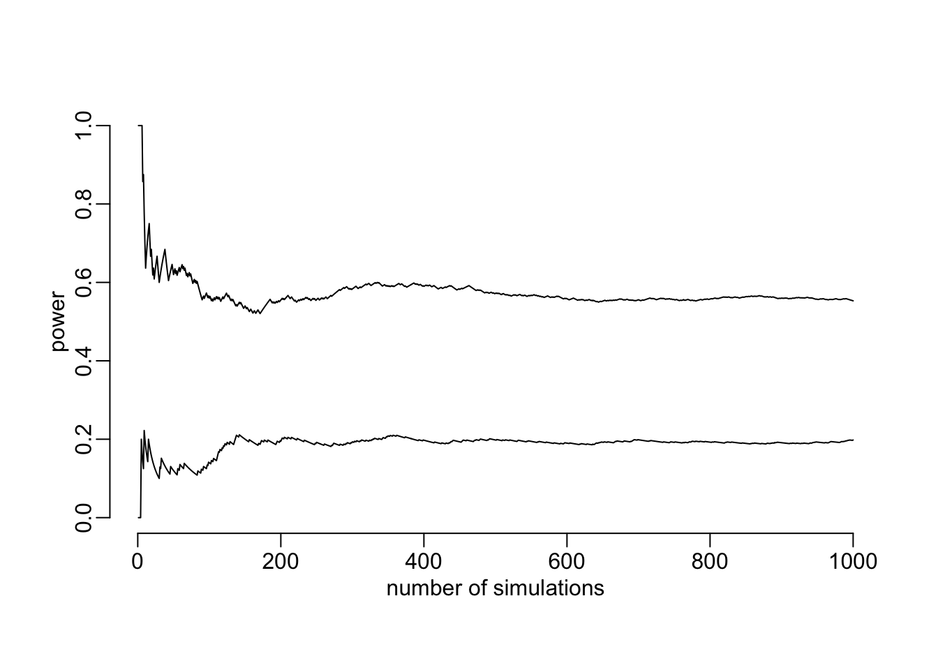
And see whether the number of simulations (1000) looks about OK (i.e. whether the power has converged):

plot(cummean(out[[1]]),
     type = "l", xlab = "number of simulations", ylab = "power", ylim = 0:1)

lines(cummean(out[[2]]))

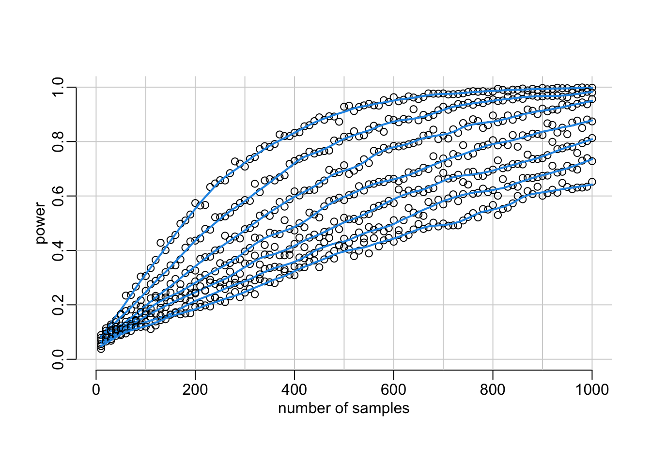
Looks about OK. Next step is the compute the power for various samples sizes (takes about 40’ on an 11-core):

samples_sizes <- seq(10, 1000, 10)

powers <- seq(0, 30, 5) |>
  map(~ mclapply(
    samples_sizes,
    function(x) decay_rate_power(p0 = .3, p1 = .1, t = 10, N = 1000,
                                 t_entry = function() runif(x, max = 10),
                                 t_exposure = function() runif(x, max = .x)),
    mc.cores = detectCores() - 1))

Let’s visualize it:

plot(NA, xlim = c(0, 1000), ylim = 0:1, xlab = "number of samples", ylab = "power")
abline2(v = seq(0, 1000, 100)); abline2(h = seq(0, 1, .2))

walk(powers,
     function(x) {
       mean_powers <- map_dbl(x, mean)
       points(samples_sizes, mean_powers)
       with(lowess(samples_sizes, mean_powers, .1), lines(x, y, col = 4, lwd = 2))})

Looking for the number of samples that gives 80% power:

power2n <- function(power,
                    data = lowess(samples_sizes, map_dbl(powers[[1]], mean), .1), ...) {
  optimize(function(xout) with(data, abs(approx(x, y, xout, ...)$y - power)),
           c(0, 1000))$minimum
}

The number of the samples needed to get a power of 80% in case there is no delay between exposure and country entry:

power2n(.8)

[1] 365.654